Run CalicoST on prostate cancer dataset
Obtain the data
We obtained the spatially resolved transcriptomics of a prostate cross section studied by Erickon et al. from EGA using accession EGAD00001008644. We ran spaceranger to get the BAM files and applied CalicoST to study the CNAs and spatial evolution of cancer across multiple spatial regions.
Compute allele counts by preprocessing: genotyping and reference-based phasing
Step 1: Download SNP and phasing panels
Download the following files to your machine.
SNP panel - 0.5GB in size. You can also choose other SNP panels from cellsnp-lite webpage.
Phasing panel- 9.0GB in size. Unzip the panel after downloading.
Step 2: Make a table for BAM files and slice IDs to jointly genotype and phase
In order to jointly genotype and phase across multiple slices, CalicoST requires a bamlist.tsv file that specifies the BAM file paths, slice IDs, and spaceranger output directories. It must be tab-deliminated, without header, and contain the following columns in order, otherwise the pipeline will report an error.
BAM file location |
slide ID |
spaceranger out directory location |
|---|
Below is the bamlist.tsv file we used for the prostate cancer data.
/u/congma/ragr-data/datasets/spatial_cna/Lundeberg_organwide/P1_spaceranger/P1_H1_2_visium/outs/possorted_genome_bam.bam        H12     /u/congma/ragr-data/datasets/spatial_cna/Lundeberg_organwide/P1_spaceranger/P1_H1_2_visium/outs/
/u/congma/ragr-data/datasets/spatial_cna/Lundeberg_organwide/P1_spaceranger/P1_H1_4_visium/outs/possorted_genome_bam.bam        H14     /u/congma/ragr-data/datasets/spatial_cna/Lundeberg_organwide/P1_spaceranger/P1_H1_4_visium/outs/
/u/congma/ragr-data/datasets/spatial_cna/Lundeberg_organwide/P1_spaceranger/P1_H1_5_visium/outs/possorted_genome_bam.bam        H15     /u/congma/ragr-data/datasets/spatial_cna/Lundeberg_organwide/P1_spaceranger/P1_H1_5_visium/outs/
/u/congma/ragr-data/datasets/spatial_cna/Lundeberg_organwide/P1_spaceranger/P1_H2_1_visium/outs/possorted_genome_bam.bam        H21     /u/congma/ragr-data/datasets/spatial_cna/Lundeberg_organwide/P1_spaceranger/P1_H2_1_visium/outs/
/u/congma/ragr-data/datasets/spatial_cna/Lundeberg_organwide/P1_spaceranger/P1_H2_5_visium/outs/possorted_genome_bam.bam        H25     /u/congma/ragr-data/datasets/spatial_cna/Lundeberg_organwide/P1_spaceranger/P1_H2_5_visium/outs/
Step 3: Make a config.yaml for snakemake preprocessing pipeline
Besides the BAM files, we also need to specify the reference SNPs and phasing panels and other running configurations. These will be specified in the config.yaml file. A template config.yaml file is available in our github. You can modify the template with paths to the references on our machine. Below is the content of config.yaml file we used.
# path to executables or their parent directories
calicost_dir: /n/fs/ragr-data/users/congma/Codes/CalicoST
eagledir: /n/fs/ragr-data/users/congma/environments/Eagle_v2.4.1

# running parameters
# samtools sort (only used when joingly calling from multiple slices)
samtools_sorting_mem: "4G"
# cellsnp-lite
UMItag: "Auto"
cellTAG: "CB"
nthreads_cellsnplite: 20
region_vcf: /n/fs/ragr-data/users/congma/references/snplist/nocpg.genome1K.phase3.SNP_AF5e4.chr1toX.hg38.vcf.gz
# Eagle phasing
phasing_panel: /n/fs/ragr-data/users/congma/references/phasing_ref/1000G_hg38
chromosomes: [1, 2, 3, 4, 5, 6, 7, 8, 9, 10, 11, 12, 13, 14, 15, 16, 17, 18, 19, 20, 21, 22]

# input
bamlist: /n/fs/ragr-data/datasets/spatial_cna/Lundeberg_organwide/P1_snps/joint_H1_245_H2_15/bamlist.tsv

# output
output_snpinfo: /n/fs/ragr-data/datasets/spatial_cna/Lundeberg_organwide/P1_snps/joint_H1_245_H2_15
Step 4: Run the proprocessing snakemake pipeline
With the input of modified config.yaml file, we run the snakemake pipeline calicost.smk as follows.
snakemake --cores <number threads> --configfile config.yaml --snakefile calicost.smk all
Key outputs of the snakemake preprocessing pipeline
In the directory specified in output_snpinfo entry of the config.yaml file, we will see the following allele count files
cell_snp_Aallele.npz: A scipy sparse matrix of number spots * number SNPs, each entry indicates the UMI counts of the first haplotype phased by Eagle2.
cell_snp_Ballele.npz: A scipy sparse matrix of number spots * number SNPs, each entry indicates the UMI counts of the second haplotype phased by Eagle2.
unique_snp_ids.npy: The ID each the SNPs, corresponding to the columns of scipy sparse matrices.
barcodes.txt: The spot barcodes (with slide IDs appended as suffix), corresponding to the rows of scipy sparse matrices.
Estimate tumor proportion per spot
Step 1: Make the configuration_purity file
To use CalicoST for inferring tumor proportion, first set up a configuration file for CalicoST to specify the input paths, output paths, and running configurations. A template configuration_purity file is available at the github repo. Modify the input/output directories from the template. We used the following configuration_purity file for estimating tumor purity on the prostate cancer data.
input_filelist : /n/fs/ragr-data/datasets/spatial_cna/Lundeberg_organwide/P1_snps/joint_H1_245_H2_15/bamlist.tsv
snp_dir : /n/fs/ragr-data/datasets/spatial_cna/Lundeberg_organwide/P1_snps/joint_H1_245_H2_15
output_dir : /n/fs/ragr-data/users/congma/Datasets/CalicoST_prostate_example/estimate_tumor_prop

# supporting files and preprocessing arguments
geneticmap_file : /n/fs/ragr-data/users/congma/Codes/CalicoST/GRCh38_resources/genetic_map_GRCh38_merged.tab.gz
hgtable_file : /n/fs/ragr-data/users/congma/Codes/CalicoST/GRCh38_resources/hgTables_hg38_gencode.txt
normalidx_file : None
tumorprop_file : None
alignment_files :
supervision_clone_file : None
filtergenelist_file : /n/fs/ragr-data/users/congma/Codes/CalicoST/GRCh38_resources/ig_gene_list.txt
filterregion_file : /n/fs/ragr-data/users/congma/Codes/CalicoST/GRCh38_resources/HLA_regions.bed
secondary_min_umi : 400
bafonly : False

# phase switch probability
nu : 1.0
logphase_shift : -2.0
npart_phasing : 3

# HMRF configurations
n_clones : 5
n_clones_rdr : 2
min_spots_per_clone : 100
min_avgumi_per_clone : 10
maxspots_pooling : 19
tumorprop_threshold : 0.7
max_iter_outer : 20
nodepotential : weighted_sum
initialization_method : rectangle
num_hmrf_initialization_start : 0
num_hmrf_initialization_end : 1
spatial_weight : 1.0
construct_adjacency_method : hexagon
construct_adjacency_w : 1.0

# HMM configurations
n_states : 7
params : smp
t : 1-1e-4
t_phaseing : 0.9999
fix_NB_dispersion : False
shared_NB_dispersion : True
fix_BB_dispersion : False
shared_BB_dispersion : True
max_iter : 30
tol : 0.0001
gmm_random_state : 0
np_threshold : 1.0
np_eventminlen : 10

# integer copy number
nonbalance_bafdist : 1.0
nondiploid_rdrdist : 10.0
For more information of the running configurations, refer to this page in the documentations.
Step 2: Run the tumor purity estimation module in CalicoST
We run the following command in terminal
# make the output directory
mkdir -p /n/fs/ragr-data/users/congma/Datasets/CalicoST_prostate_example/estimate_tumor_prop/
# run CalicoST to infer tumor purity
OMP_NUM_THREADS=1 python <CalicoST git-cloned directory>/src/calicost/estimate_tumor_proportion.py -c configuration_purity
This command takes about 1.5 hours to run and will generate an output file of loh_estimator_tumor_prop.tsv in the output directory.
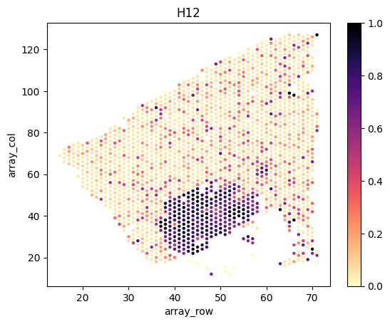
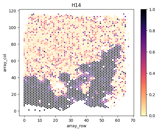
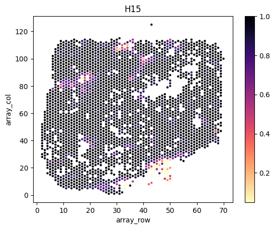
Load and visualize inferred tumor proportions
We load and visualize the estimated tumor proportions as follows.
import scanpy as sc
import numpy as np
import pandas as pd
from matplotlib import pyplot as plt
import seaborn as sns
import copy
# Modify the example_directory to be the path of the downloaded and untarred data.
example_directory = "./"

tumor_proportions = pd.read_csv(f'{example_directory}/estimate_tumor_prop/loh_estimator_tumor_prop.tsv', header=0, index_col=0, sep='\t')
tumor_proportions
| Tumor | |
|---|---|
| BARCODES | |
| AAACAAGTATCTCCCA-1_H12 | 0.050000 |
| AAACAGGGTCTATATT-1_H12 | NaN |
| AAACATTTCCCGGATT-1_H12 | 0.050000 |
| AAACCGGGTAGGTACC-1_H12 | 0.825997 |
| AAACCGTTCGTCCAGG-1_H12 | 0.940555 |
| ... | ... |
| TTGTTCAGTGTGCTAC-1_H25 | 0.050000 |
| TTGTTGTGTGTCAAGA-1_H25 | 0.188937 |
| TTGTTTCACATCCAGG-1_H25 | 0.956014 |
| TTGTTTCATTAGTCTA-1_H25 | 0.838851 |
| TTGTTTCCATACAACT-1_H25 | 0.364009 |
13344 rows × 1 columns
slice_ids = ['H12', 'H14', 'H15', 'H21', 'H25']
directory_name = ['P1_H1_2_visium', 'P1_H1_4_visium', 'P1_H1_5_visium', 'P1_H2_1_visium', 'P1_H2_5_visium']
for i,s in enumerate(slice_ids):
# load spatial locations
# note that scanpy is incompatible with the latest tissue_positions.csv file, we directly load the positions as pandas data frame
df = pd.read_csv(f'{example_directory}/data/{directory_name[i]}/spatial/tissue_positions.csv', header=0, index_col=0, sep=',')
print(df.head())
# combine the position data frame with the tumor proportion dataframe
slice_tumor_proportions = tumor_proportions[tumor_proportions.index.str.endswith(s)]
df = df.join( slice_tumor_proportions.rename(index=lambda x:x.split("_")[0]) )
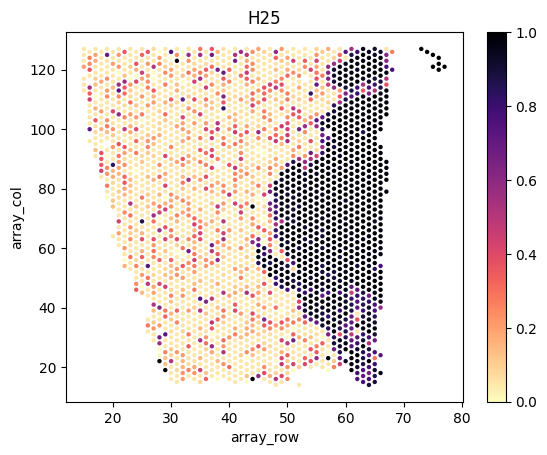
# plot
fig, axes = plt.subplots(1, 1, facecolor='white')
sns.scatterplot(x=df.array_row, y=df.array_col, hue=df.Tumor, palette='magma_r', linewidth=0, s=10, legend=False, ax=axes)
norm = plt.Normalize(np.nanmin(df.Tumor.values), np.nanmax(df.Tumor.values))
axes.figure.colorbar( plt.cm.ScalarMappable(cmap='magma_r', norm=norm), ax=axes )
axes.set_title(s)
plt.show()
                    in_tissue  array_row  array_col  pxl_row_in_fullres  \
barcode
ACGCCTGACACGCGCT-1          0          0          0                1466
TACCGATCCAACACTT-1          0          1          1                1592
ATTAAAGCGGACGAGC-1          0          0          2                1466
GATAAGGGACGATTAG-1          0          1          3                1592
GTGCAAATCACCAATA-1          0          0          4                1466

                    pxl_col_in_fullres
barcode
ACGCCTGACACGCGCT-1                1298
TACCGATCCAACACTT-1                1370
ATTAAAGCGGACGAGC-1                1443
GATAAGGGACGATTAG-1                1515
GTGCAAATCACCAATA-1                1588
                    in_tissue  array_row  array_col  pxl_row_in_fullres  \
barcode
ACGCCTGACACGCGCT-1          0          0          0                1831
TACCGATCCAACACTT-1          0          1          1                1983
ATTAAAGCGGACGAGC-1          0          0          2                1831
GATAAGGGACGATTAG-1          0          1          3                1983
GTGCAAATCACCAATA-1          0          0          4                1831

                    pxl_col_in_fullres
barcode
ACGCCTGACACGCGCT-1                1544
TACCGATCCAACACTT-1                1631
ATTAAAGCGGACGAGC-1                1718
GATAAGGGACGATTAG-1                1805
GTGCAAATCACCAATA-1                1892
                    in_tissue  array_row  array_col  pxl_row_in_fullres  \
barcode
ACGCCTGACACGCGCT-1          0          0          0                1593
TACCGATCCAACACTT-1          0          1          1                1720
ATTAAAGCGGACGAGC-1          0          0          2                1593
GATAAGGGACGATTAG-1          0          1          3                1719
GTGCAAATCACCAATA-1          0          0          4                1593

                    pxl_col_in_fullres
barcode
ACGCCTGACACGCGCT-1                1172
TACCGATCCAACACTT-1                1245
ATTAAAGCGGACGAGC-1                1317
GATAAGGGACGATTAG-1                1390
GTGCAAATCACCAATA-1                1462
                    in_tissue  array_row  array_col  pxl_row_in_fullres  \
barcode
ACGCCTGACACGCGCT-1          0          0          0                1830
TACCGATCCAACACTT-1          0          1          1                1982
ATTAAAGCGGACGAGC-1          0          0          2                1831
GATAAGGGACGATTAG-1          0          1          3                1982
GTGCAAATCACCAATA-1          0          0          4                1831

                    pxl_col_in_fullres
barcode
ACGCCTGACACGCGCT-1                1523
TACCGATCCAACACTT-1                1610
ATTAAAGCGGACGAGC-1                1697
GATAAGGGACGATTAG-1                1784
GTGCAAATCACCAATA-1                1871

                    in_tissue  array_row  array_col  pxl_row_in_fullres  \
barcode
ACGCCTGACACGCGCT-1          0          0          0                1948
TACCGATCCAACACTT-1          0          1          1                2100
ATTAAAGCGGACGAGC-1          0          0          2                1948
GATAAGGGACGATTAG-1          0          1          3                2100
GTGCAAATCACCAATA-1          0          0          4                1947

                    pxl_col_in_fullres
barcode
ACGCCTGACACGCGCT-1                1441
TACCGATCCAACACTT-1                1529
ATTAAAGCGGACGAGC-1                1616
GATAAGGGACGATTAG-1                1705
GTGCAAATCACCAATA-1                1791
Run CalicoST to infer CNAs and cancer clones based on estimated tumor proportions
Step 1: Create a configuration file for CalicoST
The configuration file for CalicoST, configuration_cna_multi, specifies the input/output paths and the running parameters. It is very similar to the configutation_purity file except that (1) it uses a different output directory, and (2)the “tumorprop_file” entry is now replaced with the output of the inferred tumor purity. Below is the configuration_cna_multi file we used.
input_filelist : /n/fs/ragr-data/datasets/spatial_cna/Lundeberg_organwide/P1_snps/joint_H1_245_H2_15/bamlist.tsv
snp_dir : /n/fs/ragr-data/datasets/spatial_cna/Lundeberg_organwide/P1_snps/joint_H1_245_H2_15
output_dir : /n/fs/ragr-data/users/congma/Datasets/CalicoST_prostate_example/calicost

# supporting files and preprocessing arguments
geneticmap_file : /n/fs/ragr-data/users/congma/Codes/CalicoST/GRCh38_resources/genetic_map_GRCh38_merged.tab.gz
hgtable_file : /n/fs/ragr-data/users/congma/Codes/CalicoST/GRCh38_resources/hgTables_hg38_gencode.txt
normalidx_file : None
tumorprop_file : /n/fs/ragr-data/users/congma/Datasets/CalicoST_prostate_example/estimate_tumor_prop/loh_estimator_tumor_prop.tsv
alignment_files :
supervision_clone_file : None
filtergenelist_file : /n/fs/ragr-data/users/congma/Codes/CalicoST/GRCh38_resources/ig_gene_list.txt
filterregion_file : /n/fs/ragr-data/users/congma/Codes/CalicoST/GRCh38_resources/HLA_regions.bed
secondary_min_umi : 400
bafonly : False

# phase switch probability
nu : 1.0
logphase_shift : -2.0
npart_phasing : 3

# HMRF configurations
n_clones : 5
n_clones_rdr : 2
min_spots_per_clone : 100
min_avgumi_per_clone : 10
maxspots_pooling : 19
tumorprop_threshold : 0.7
max_iter_outer : 20
nodepotential : weighted_sum
initialization_method : rectangle
num_hmrf_initialization_start : 0
num_hmrf_initialization_end : 1
spatial_weight : 1.0
construct_adjacency_method : hexagon
construct_adjacency_w : 1.0

# HMM configurations
n_states : 7
params : smp
t : 1-1e-4
t_phaseing : 0.9999
fix_NB_dispersion : False
shared_NB_dispersion : True
fix_BB_dispersion : False
shared_BB_dispersion : True
max_iter : 30
tol : 0.0001
gmm_random_state : 0
np_threshold : 1.0
np_eventminlen : 10

# integer copy number
nonbalance_bafdist : 1.0
nondiploid_rdrdist : 10.0
Step 2: Run the CalicoST to infer CNAs and clones
We ran the following command.
# create output directory
mkdir -p /n/fs/ragr-data/users/congma/Datasets/CalicoST_prostate_example/calicost
# run CalicoST
OMP_NUM_THREADS=1 python <CalicoST directory>/src/calicost/calicost_main.py -c configuration_cna_multi
This command takes about 8h to finish.
Load CalicoST-generated result tables
<output_dir>/clone5_rectangle0_w1.0/clone_labels.tsv stores the inferred cancer clones for each spot. Note that spots with a low tumor purity will also be assigned to a cancer clone, despite that the inferred cancer clone label is not very meaningful for those nearly normal spots.
df = pd.read_csv(f"{example_directory}/calicost/clone5_rectangle0_w1.0/clone_labels.tsv", header=0, index_col=0, sep='\t')
df
| clone_label | tumor_proportion | |
|---|---|---|
| BARCODES | ||
| AAACAAGTATCTCCCA-1_H12 | 3 | 0.050000 |
| AAACAGGGTCTATATT-1_H12 | 3 | NaN |
| AAACATTTCCCGGATT-1_H12 | 3 | 0.050000 |
| AAACCGGGTAGGTACC-1_H12 | 3 | 0.825997 |
| AAACCGTTCGTCCAGG-1_H12 | 3 | 0.940555 |
| ... | ... | ... |
| TTGTTCAGTGTGCTAC-1_H25 | 2 | 0.050000 |
| TTGTTGTGTGTCAAGA-1_H25 | 2 | 0.188937 |
| TTGTTTCACATCCAGG-1_H25 | 1 | 0.956014 |
| TTGTTTCATTAGTCTA-1_H25 | 1 | 0.838851 |
| TTGTTTCCATACAACT-1_H25 | 2 | 0.364009 |
13344 rows × 2 columns
<output_dir>/clone5_rectangle0_w1.0/cnv_seglevel.tsv stores the allele-specific copy numbers of each genome bin within each clone. Each row is a genome bin, the columns containing the chromosome, start, and end position of the genome bin, and the inferred the A and B allele copy number within each cancer clone.
df = pd.read_csv(f"{example_directory}/calicost/clone5_rectangle0_w1.0/cnv_seglevel.tsv", header=0, index_col=None, sep='\t')
df
| CHR | START | END | clone1 A | clone1 B | clone2 A | clone2 B | clone3 A | clone3 B | clone4 A | clone4 B | clone5 A | clone5 B | |
|---|---|---|---|---|---|---|---|---|---|---|---|---|---|
| 0 | 1 | 89295 | 1419136 | 1 | 1 | 1 | 1 | 1 | 1 | 1 | 1 | 1 | 1 |
| 1 | 1 | 1434861 | 1440568 | 1 | 1 | 1 | 1 | 1 | 1 | 1 | 1 | 1 | 1 |
| 2 | 1 | 1449689 | 1496123 | 1 | 1 | 1 | 1 | 1 | 1 | 1 | 1 | 1 | 1 |
| 3 | 1 | 1512162 | 1721078 | 1 | 1 | 1 | 1 | 1 | 1 | 1 | 1 | 1 | 1 |
| 4 | 1 | 1724838 | 2308568 | 1 | 1 | 1 | 1 | 1 | 1 | 1 | 1 | 1 | 1 |
| ... | ... | ... | ... | ... | ... | ... | ... | ... | ... | ... | ... | ... | ... |
| 2255 | 22 | 46360834 | 48898361 | 1 | 1 | 1 | 1 | 1 | 1 | 1 | 1 | 1 | 1 |
| 2256 | 22 | 49773283 | 49963978 | 1 | 1 | 1 | 1 | 1 | 1 | 1 | 1 | 1 | 1 |
| 2257 | 22 | 50089879 | 50180213 | 1 | 1 | 1 | 1 | 1 | 1 | 1 | 1 | 1 | 1 |
| 2258 | 22 | 50185915 | 50292030 | 1 | 1 | 1 | 1 | 1 | 1 | 1 | 1 | 1 | 1 |
| 2259 | 22 | 50309030 | 50783625 | 1 | 1 | 1 | 1 | 1 | 1 | 1 | 1 | 1 | 1 |
2260 rows × 13 columns
<output_dir>/clone5_rectangle0_w1.0/cnv_genelevel.tsv stores the allele-specific copy number for each gene. The copy number per gene is derived from projecting the allele-specific copy numbers of each genome bin to the spanned genes that have enough expression to be retained after CalicoST gene filtering step.
df = pd.read_csv(f"{example_directory}/calicost/clone5_rectangle0_w1.0/cnv_genelevel.tsv", header=0, index_col=None, sep='\t')
df
| gene | clone1 A | clone1 B | clone2 A | clone2 B | clone3 A | clone3 B | clone4 A | clone4 B | clone5 A | clone5 B | |
|---|---|---|---|---|---|---|---|---|---|---|---|
| 0 | AL627309.1 | 1 | 1 | 1 | 1 | 1 | 1 | 1 | 1 | 1 | 1 |
| 1 | AL627309.5 | 1 | 1 | 1 | 1 | 1 | 1 | 1 | 1 | 1 | 1 |
| 2 | LINC01409 | 1 | 1 | 1 | 1 | 1 | 1 | 1 | 1 | 1 | 1 |
| 3 | LINC01128 | 1 | 1 | 1 | 1 | 1 | 1 | 1 | 1 | 1 | 1 |
| 4 | LINC00115 | 1 | 1 | 1 | 1 | 1 | 1 | 1 | 1 | 1 | 1 |
| ... | ... | ... | ... | ... | ... | ... | ... | ... | ... | ... | ... |
| 15035 | CHKB-DT | 1 | 1 | 1 | 1 | 1 | 1 | 1 | 1 | 1 | 1 |
| 15036 | MAPK8IP2 | 1 | 1 | 1 | 1 | 1 | 1 | 1 | 1 | 1 | 1 |
| 15037 | ARSA | 1 | 1 | 1 | 1 | 1 | 1 | 1 | 1 | 1 | 1 |
| 15038 | SHANK3 | 1 | 1 | 1 | 1 | 1 | 1 | 1 | 1 | 1 | 1 |
| 15039 | RABL2B | 1 | 1 | 1 | 1 | 1 | 1 | 1 | 1 | 1 | 1 |
15040 rows × 11 columns
Visualize CalicoST-generated plots
Once CalicoST is finished running, it generates the plots of spatial organization of clones and allele-specific copy numbers. The plots are in PDF format and can be directly viewed. Below, we load the PDF plots in this notebook for easy visualization.
from wand.image import Image as WImage
img = WImage(filename=f"{example_directory}/calicost/clone5_rectangle0_w1.0/plots/clone_spatial.pdf", resolution=100)
img

# allele-specific copy numbers of each clone (the color scheme is the same as Fig2c
img = WImage(filename=f"{example_directory}/calicost/clone5_rectangle0_w1.0/plots/acn_genome.pdf", resolution=120)
img

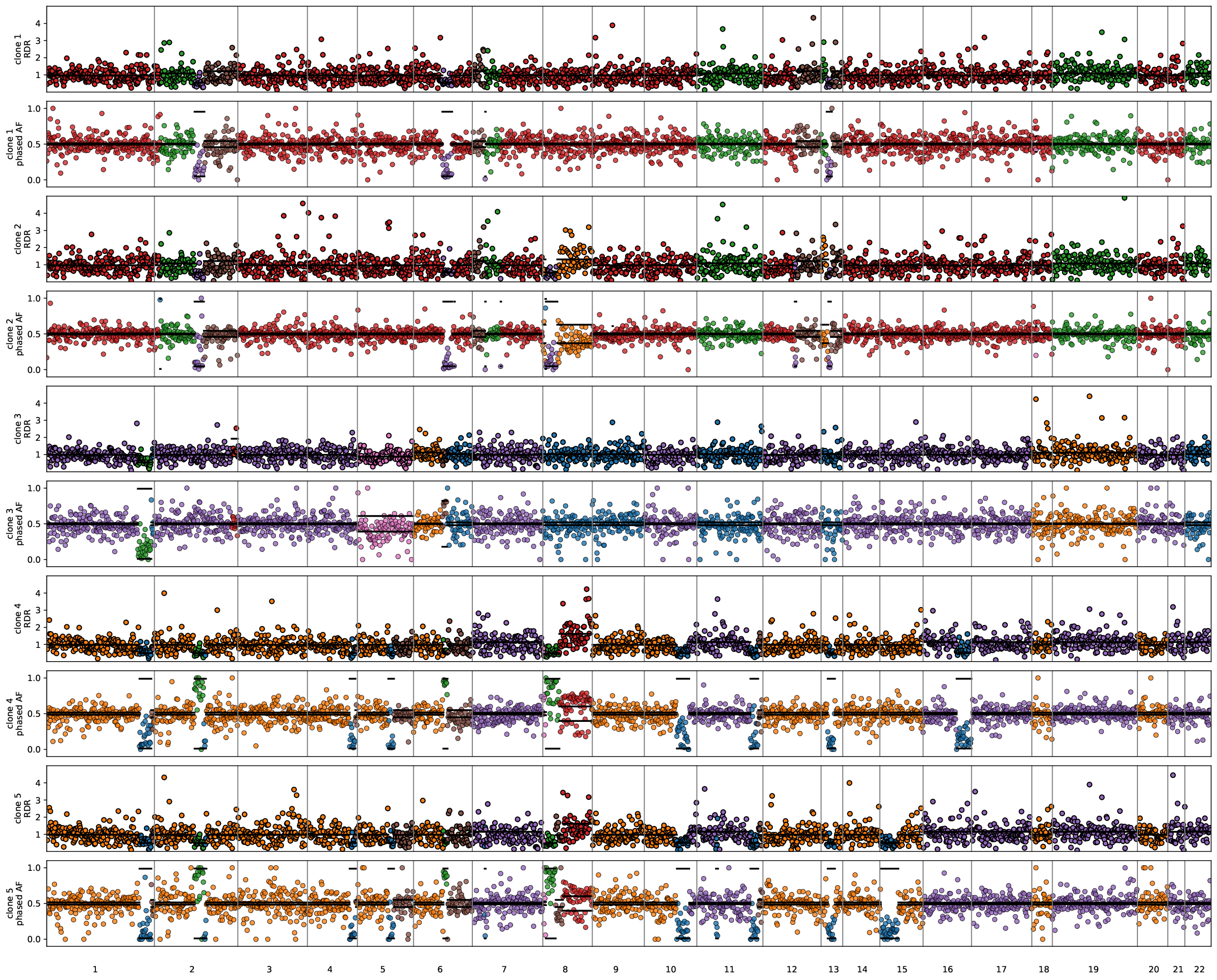
# RDR-BAF plot along the genome for each clone
img = WImage(filename=f"{example_directory}/calicost/clone5_rectangle0_w1.0/plots/rdr_baf_defaultcolor.pdf", resolution=120)
img
Reconstruct tumor phylogeny and phylogeography
We use an existing phylogeny reconstruction method, Startle by Sashittal et al, to infer a phylogeny of CalicoST-inferred cancer clones. To reconstruct a phylogeny based CalicoST results of the first random initialization, run the following command in shell:
mkdir calicost/phylogeny_clone5_rectangle0_w1.0
python <CalicoST code directory>/src/calicost/phylogeny_startle.py -c calicost/clone5_rectangle0_w1.0 -s <startle executable path> -o calicost/phylogeny_clone5_rectangle0_w1.0/
The above run of Startle will produce a plain-text file calicost/phylogeny_clone5_rectangle0_w1.0/loh_tree.newick that encodes phylogeny tree with leaf nodes as CalicoST-inferred clones. We load the tree file as follows.
with open(f"{example_directory}/calicost/phylogeny_clone5_rectangle0_w1.0/loh_tree.newick", 'r') as fp:
    print( fp.readlines() )
['((clone1:0,clone2:3):4,(clone3:1,(clone4:3,clone5:3):9):2);']
Now we project the phylogenetic tree in space to get a phylogeography. Before getting the phylogeography, we note that we currently don’t have the relative positioning among the five slices yet. We manually place the five slices according to Fig 1b in the original publication by Erickon et al., and transform the x/y coordinate in the tissue_positions.csv file according to the new positioning.
# load coordinates and inferred cancer clones
coords = []
for i,s in enumerate(slice_ids):
    # load spatial locations
    # note that scanpy is incompatible with the latest tissue_positions.csv file, we directly load the positions as pandas data frame
    df = pd.read_csv(f'{example_directory}/data/{directory_name[i]}/spatial/tissue_positions.csv', header=0, index_col=0, sep=',')
    df.index = df.index + "_" + s
    df['slice_id'] = s
    coords.append( df )

coords = pd.concat(coords)

# combine with the cancer clone table
df = pd.read_csv(f"{example_directory}/calicost/clone5_rectangle0_w1.0/clone_labels.tsv", header=0, index_col=0, sep='\t')
df.clone_label = 'clone' + df.clone_label.astype(str)
coords = coords.join(df)

# remove spots that are not assigned to clones by CalicoST (filtered out due to low UMI count or SNP-covering UMI count)
coords = coords[coords.clone_label.notnull()]
coords
| in_tissue | array_row | array_col | pxl_row_in_fullres | pxl_col_in_fullres | slice_id | clone_label | tumor_proportion | |
|---|---|---|---|---|---|---|---|---|
| barcode | ||||||||
| TCCTTCAGTGGTCGAA-1_H12 | 1 | 15 | 69 | 3366 | 6308 | H12 | clone3 | 0.050000 |
| GCGTCGAAATGTCGGT-1_H12 | 1 | 17 | 65 | 3618 | 6018 | H12 | clone3 | 0.132391 |
| AACTGATATTAGGCCT-1_H12 | 1 | 16 | 66 | 3492 | 6090 | H12 | clone3 | 0.050000 |
| CGAGCTGGGCTTTAGG-1_H12 | 1 | 17 | 67 | 3618 | 6163 | H12 | clone3 | 0.050000 |
| GGGTGTTTCAGCTATG-1_H12 | 1 | 16 | 68 | 3492 | 6236 | H12 | clone3 | 0.050000 |
| ... | ... | ... | ... | ... | ... | ... | ... | ... |
| ATGGCCCGAAAGGTTA-1_H25 | 1 | 76 | 120 | 13480 | 12001 | H25 | clone2 | 1.000000 |
| CGTAATATGGCCCTTG-1_H25 | 1 | 77 | 121 | 13632 | 12089 | H25 | clone2 | 1.000000 |
| AGAGTCTTAATGAAAG-1_H25 | 1 | 76 | 122 | 13480 | 12176 | H25 | clone2 | 1.000000 |
| ATTGAATTCCCTGTAG-1_H25 | 1 | 76 | 124 | 13479 | 12351 | H25 | clone2 | 1.000000 |
| TTGAAGTGCATCTACA-1_H25 | 1 | 77 | 127 | 13630 | 12615 | H25 | clone2 | NaN |
13344 rows × 8 columns
def flip_axis(coords, axis):
    max_x = np.max(coords[:,axis])
    min_x = np.min(coords[:,axis])
    tmp_coords = copy.copy(coords)
    tmp_coords[:,axis] = min_x + max_x - coords[:,axis]
    return tmp_coords


def rotate_by_angle(coords, angle):
    theta = angle / 180 * np.pi
    R = np.array([ [np.cos(theta), -np.sin(theta)], [np.sin(theta), np.cos(theta)]] )
    mean_coords = np.mean(coords, axis=0)
    return (coords - mean_coords.reshape(1,-1)) @ R + mean_coords.reshape(1,-1)
adjusted_coords = copy.copy(coords[['array_row', 'array_col']].values)
# scale y coordinate so that the hexagon is not squeezed on one direction
adjusted_coords[:,0] = adjusted_coords[:,0] * np.sqrt(3)
# shift x and y coordinate to start from 0 for each slice
for s,sname in enumerate(slice_ids):
    index = np.where(coords.slice_id.values == sname)[0]
    adjusted_coords[index,0] -= np.min(adjusted_coords[index,0])
    adjusted_coords[index,1] -= np.min(adjusted_coords[index,1])


# position in number of cubes
cube_length = min( np.max(adjusted_coords[:,0]), np.max(adjusted_coords[:,1]) )
sample_cube_pos = np.array([ [2,0], #H12
                             [4, 0.2], #H14
                             [5,0.5], #H15
                             [0,1], #H21
                             [5,1.5] ]) #H25

swap_x_y = [False, True, True, False, True]
rotation_angle = [15,-5,-5,0,-5] # H12, H14, H15, H21, H25

full_adj_coords = np.zeros(adjusted_coords.shape)
for s,sname in enumerate(slice_ids):
    index = np.where(coords.slice_id.values == sname)[0]
    if swap_x_y[s]:
        tmp_coords = np.vstack([adjusted_coords[index,1],adjusted_coords[index,0]]).T
        if sname != "H25":
            tmp_coords = flip_axis(tmp_coords, axis=0 )
        tmp_coords = flip_axis(tmp_coords, axis=1)
        full_adj_coords[index,:] = tmp_coords + cube_length * sample_cube_pos[s]
    else:
        full_adj_coords[index,:] = adjusted_coords[index,:] + cube_length * sample_cube_pos[s]

    full_adj_coords[index,:] = rotate_by_angle(full_adj_coords[index,:], rotation_angle[s])

coords['final_x'] = full_adj_coords[:,0]
coords['final_y'] = full_adj_coords[:,1]
coords
| in_tissue | array_row | array_col | pxl_row_in_fullres | pxl_col_in_fullres | slice_id | clone_label | tumor_proportion | final_x | final_y | |
|---|---|---|---|---|---|---|---|---|---|---|
| barcode | ||||||||||
| TCCTTCAGTGGTCGAA-1_H12 | 1 | 15 | 69 | 3366 | 6308 | H12 | clone3 | 0.050000 | 238.417652 | 74.069483 |
| GCGTCGAAATGTCGGT-1_H12 | 1 | 17 | 65 | 3618 | 6018 | H12 | clone3 | 0.132391 | 241.246079 | 69.170504 |
| AACTGATATTAGGCCT-1_H12 | 1 | 16 | 66 | 3492 | 6090 | H12 | clone3 | 0.050000 | 239.573047 | 70.654068 |
| CGAGCTGGGCTTTAGG-1_H12 | 1 | 17 | 67 | 3618 | 6163 | H12 | clone3 | 0.050000 | 241.763717 | 71.102355 |
| GGGTGTTTCAGCTATG-1_H12 | 1 | 16 | 68 | 3492 | 6236 | H12 | clone3 | 0.050000 | 240.090685 | 72.585919 |
| ... | ... | ... | ... | ... | ... | ... | ... | ... | ... | ... |
| ATGGCCCGAAAGGTTA-1_H25 | 1 | 76 | 120 | 13480 | 12001 | H25 | clone2 | 1.000000 | 700.743520 | 183.090182 |
| CGTAATATGGCCCTTG-1_H25 | 1 | 77 | 121 | 13632 | 12089 | H25 | clone2 | 1.000000 | 701.914026 | 181.184948 |
| AGAGTCTTAATGAAAG-1_H25 | 1 | 76 | 122 | 13480 | 12176 | H25 | clone2 | 1.000000 | 702.735909 | 183.264493 |
| ATTGAATTCCCTGTAG-1_H25 | 1 | 76 | 124 | 13479 | 12351 | H25 | clone2 | 1.000000 | 704.728299 | 183.438805 |
| TTGAAGTGCATCTACA-1_H25 | 1 | 77 | 127 | 13630 | 12615 | H25 | clone2 | NaN | 707.891194 | 181.707882 |
13344 rows × 10 columns
import calicost.utils_plotting

fig = calicost.utils_plotting.plot_individual_spots_in_space(full_adj_coords, coords.clone_label, coords.tumor_proportion, base_width=10, base_height=5)
plt.gca().invert_yaxis()
fig.show()
/n/fs/ragr-data/users/congma/temp/CalicoST/src/calicost/utils_plotting.py:1404: FutureWarning: Series.__getitem__ treating keys as positions is deprecated. In a future version, integer keys will always be treated as labels (consistent with DataFrame behavior). To access a value by position, use `ser.iloc[pos]`
  quantile_colors = this_full_cmap(np.array([0, np.min(copy_single_tumor_prop[idx]), np.max(copy_single_tumor_prop[idx]), 1]))
/n/fs/ragr-data/users/congma/temp/CalicoST/src/calicost/utils_plotting.py:1407: FutureWarning: Series.__getitem__ treating keys as positions is deprecated. In a future version, integer keys will always be treated as labels (consistent with DataFrame behavior). To access a value by position, use `ser.iloc[pos]`
  seaborn.scatterplot(x=shifted_coords[idx,0], y=-shifted_coords[idx,1], s=10, hue=copy_single_tumor_prop[idx], palette=this_cmap, linewidth=0, legend=None, ax=axes)

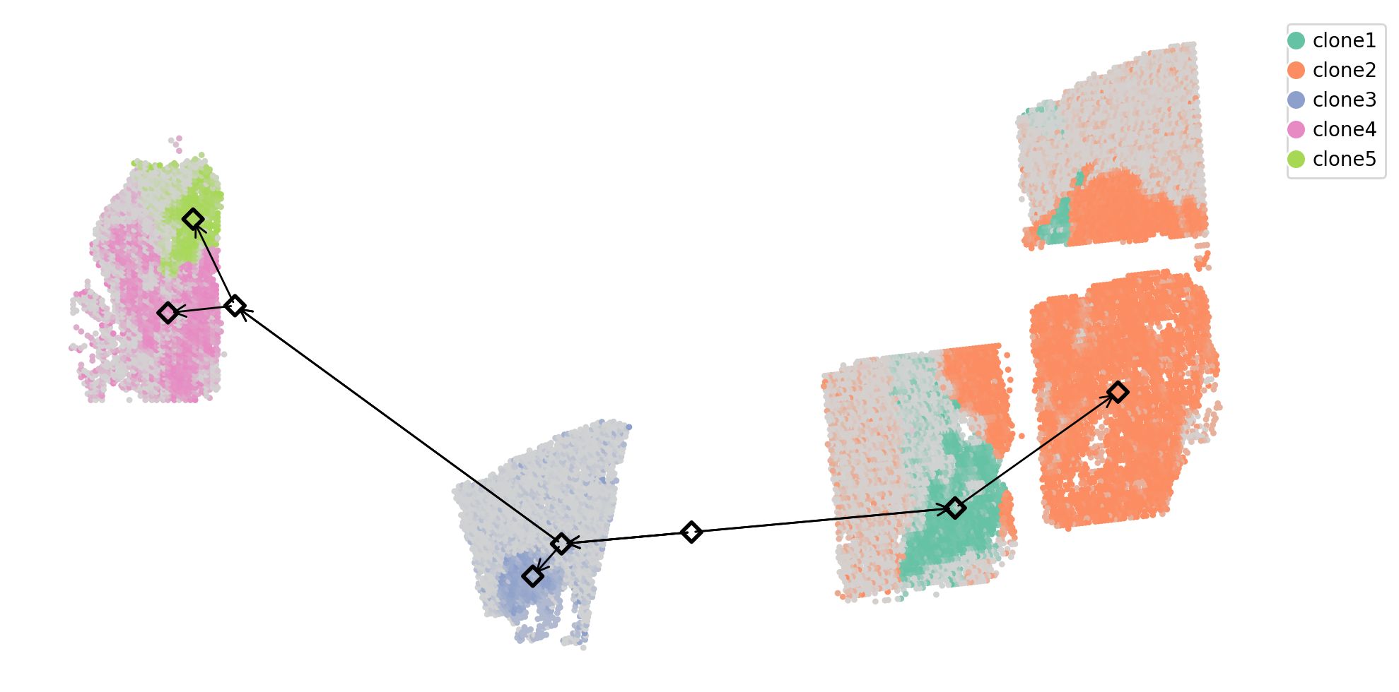
Now we project the phylogeny to the space of coords[[‘final_x’, ‘final_y’]] and infer ancestor locations using a Gaussian diffusion model.
import calicost.phylogeography

newick_file = f"{example_directory}/calicost/phylogeny_clone5_rectangle0_w1.0/loh_tree.newick"
t = calicost.phylogeography.project_phylogeneny_space(newick_file, coords[['final_x', 'final_y']].values, coords.clone_label.values,
                              single_tumor_prop=coords.tumor_proportion.values, sample_list=slice_ids, sample_ids=coords.slice_id.values)

print( t )
root node is ancestor1_2_3_4_5
a list of leaf nodes: ['clone1', 'clone2', 'clone3', 'clone4', 'clone5']
a list of internal nodes: ['ancestor1_2_3_4_5', 'ancestor1_2', 'ancestor3_4_5', 'ancestor4_5']

      /-clone1
   /-|
  |   \-clone2
--|
  |   /-clone3
   \-|
     |   /-clone4
      \-|
         \-clone5
# plot clones in space with the phylogeography

fig = calicost.utils_plotting.plot_individual_spots_in_space(full_adj_coords, coords.clone_label, coords.tumor_proportion, base_width=10, base_height=5)
axes = plt.gca()

# clone centers + ancestors
for node in t.traverse():
    axes.scatter( node.x, -node.y, marker="D", linewidth=2, edgecolor='black', facecolor="None", s=50)

# edges
for node in t.iter_leaves():
    while not node.is_root():
        p = node.up
        if np.abs(node.x - p.x) + np.abs(node.y - p.y) > 1:
            axes.annotate("", xy=(node.x, -node.y), xytext=(p.x, -p.y), arrowprops=dict(mutation_scale=15, lw=1, arrowstyle="->", color="black"))
        node = p

axes.invert_yaxis()
fig.show()
/n/fs/ragr-data/users/congma/temp/CalicoST/src/calicost/utils_plotting.py:1404: FutureWarning: Series.__getitem__ treating keys as positions is deprecated. In a future version, integer keys will always be treated as labels (consistent with DataFrame behavior). To access a value by position, use `ser.iloc[pos]`
  quantile_colors = this_full_cmap(np.array([0, np.min(copy_single_tumor_prop[idx]), np.max(copy_single_tumor_prop[idx]), 1]))
/n/fs/ragr-data/users/congma/temp/CalicoST/src/calicost/utils_plotting.py:1407: FutureWarning: Series.__getitem__ treating keys as positions is deprecated. In a future version, integer keys will always be treated as labels (consistent with DataFrame behavior). To access a value by position, use `ser.iloc[pos]`
  seaborn.scatterplot(x=shifted_coords[idx,0], y=-shifted_coords[idx,1], s=10, hue=copy_single_tumor_prop[idx], palette=this_cmap, linewidth=0, legend=None, ax=axes)
/n/fs/ragr-data/users/congma/temp/CalicoST/src/calicost/utils_plotting.py:1404: FutureWarning: Series.__getitem__ treating keys as positions is deprecated. In a future version, integer keys will always be treated as labels (consistent with DataFrame behavior). To access a value by position, use `ser.iloc[pos]`
  quantile_colors = this_full_cmap(np.array([0, np.min(copy_single_tumor_prop[idx]), np.max(copy_single_tumor_prop[idx]), 1]))
/n/fs/ragr-data/users/congma/temp/CalicoST/src/calicost/utils_plotting.py:1407: FutureWarning: Series.__getitem__ treating keys as positions is deprecated. In a future version, integer keys will always be treated as labels (consistent with DataFrame behavior). To access a value by position, use `ser.iloc[pos]`
  seaborn.scatterplot(x=shifted_coords[idx,0], y=-shifted_coords[idx,1], s=10, hue=copy_single_tumor_prop[idx], palette=this_cmap, linewidth=0, legend=None, ax=axes)
/n/fs/ragr-data/users/congma/temp/CalicoST/src/calicost/utils_plotting.py:1404: FutureWarning: Series.__getitem__ treating keys as positions is deprecated. In a future version, integer keys will always be treated as labels (consistent with DataFrame behavior). To access a value by position, use `ser.iloc[pos]`
  quantile_colors = this_full_cmap(np.array([0, np.min(copy_single_tumor_prop[idx]), np.max(copy_single_tumor_prop[idx]), 1]))
/n/fs/ragr-data/users/congma/temp/CalicoST/src/calicost/utils_plotting.py:1407: FutureWarning: Series.__getitem__ treating keys as positions is deprecated. In a future version, integer keys will always be treated as labels (consistent with DataFrame behavior). To access a value by position, use `ser.iloc[pos]`
  seaborn.scatterplot(x=shifted_coords[idx,0], y=-shifted_coords[idx,1], s=10, hue=copy_single_tumor_prop[idx], palette=this_cmap, linewidth=0, legend=None, ax=axes)
/n/fs/ragr-data/users/congma/temp/CalicoST/src/calicost/utils_plotting.py:1404: FutureWarning: Series.__getitem__ treating keys as positions is deprecated. In a future version, integer keys will always be treated as labels (consistent with DataFrame behavior). To access a value by position, use `ser.iloc[pos]`
  quantile_colors = this_full_cmap(np.array([0, np.min(copy_single_tumor_prop[idx]), np.max(copy_single_tumor_prop[idx]), 1]))
/n/fs/ragr-data/users/congma/temp/CalicoST/src/calicost/utils_plotting.py:1407: FutureWarning: Series.__getitem__ treating keys as positions is deprecated. In a future version, integer keys will always be treated as labels (consistent with DataFrame behavior). To access a value by position, use `ser.iloc[pos]`
  seaborn.scatterplot(x=shifted_coords[idx,0], y=-shifted_coords[idx,1], s=10, hue=copy_single_tumor_prop[idx], palette=this_cmap, linewidth=0, legend=None, ax=axes)
/n/fs/ragr-data/users/congma/temp/CalicoST/src/calicost/utils_plotting.py:1404: FutureWarning: Series.__getitem__ treating keys as positions is deprecated. In a future version, integer keys will always be treated as labels (consistent with DataFrame behavior). To access a value by position, use `ser.iloc[pos]`
  quantile_colors = this_full_cmap(np.array([0, np.min(copy_single_tumor_prop[idx]), np.max(copy_single_tumor_prop[idx]), 1]))
/n/fs/ragr-data/users/congma/temp/CalicoST/src/calicost/utils_plotting.py:1407: FutureWarning: Series.__getitem__ treating keys as positions is deprecated. In a future version, integer keys will always be treated as labels (consistent with DataFrame behavior). To access a value by position, use `ser.iloc[pos]`
  seaborn.scatterplot(x=shifted_coords[idx,0], y=-shifted_coords[idx,1], s=10, hue=copy_single_tumor_prop[idx], palette=this_cmap, linewidth=0, legend=None, ax=axes)