Run CalicoST on a simulated data
Download the data
We applied CalicoST on a small simulated data provided by examples/simulated_example.tar.gz from the github, which contains the following files/directories:
simulated_example
outs: simulated transcript count matrix and spatial coordinates
snpinfo: parsed allele count matrix
Untar the data by
tar -xzvf <CalicoST git-cloned directory>/examples/simulated_example.tar.gz
Run CalicoST to infer CNAs and cancer clones assuming spots are purely tumor or purely normal
To run CalicoST, we first copy configuration_cna file provided by CalicoST github to the example directory.
cd simulated_example
cp <CalicoST git-cloned directory>/configuration_cna ./
Then we modify the following paths in the copied configuration_cna file:
spaceranger_diris path to theoutsdirectory of the downloaded data.snp_diris the path to thesnp_infodirectory of the downloaded data.output_diris the output directory for CalicoST to write the inferred clones and CNAs. It must be an existing directory.
We keep the default values for other parameters in configuration_cna file, while refer to this parameter specification for more details if parameter tuning is needed for other samples.
Now we use CalicoST to infer clones and allele-specific CNAs by running the following command in terminal
OMP_NUM_THREADS=1 python <CalicoST git-cloned directory>/src/calicost/calicost_main.py -c configuration_cna
It takes about 2h to run on this simulated data. When finished, the CalicoST output directory <output_dir> will contain the following files:
<output_dir>/clone3_rectangle0_w1.0/clone_labels.tsvstore the inferred cancer clones;<output_dir>/clone3_rectangle0_w1.0/cnv_seglevel.tsvstore the inferred allele-specific copy number profile per genomic segment;<output_dir>/clone3_rectangle0_w1.0/cnv_genelevel.tsvstore the inferred allele-specific copy numbers projected to expressed genes;<output_dir>/clone3_rectangle0_w1.0/cnv_diploid*,calicost/clone3_rectangle0_w1.0/cnv_triploid*,calicost/clone3_rectangle0_w1.0/cnv_tetraploid*store an additional version of integer allele-specific copy numbers when enforcing the ploidy to be diploid, triploid, and tetraploid. Experienced users can decide which ploidy to use based on prior knowledge or based on the rdr-baf plots.<output_dir>/clone3_rectangle0_w1.0/plots/store the plots corresponding to the spatial organization of inferred cancer clones and allele-specific copy numbers along the genome for each clone.
Load the results of CalicoST
Load the inferred cancer clones <output_dir>/clone3_rectangle0_w1.0/clone_labels.tsv by pandas.
import numpy as np
import pandas as pd

output_dir = "."
df_clones = pd.read_csv(f"{output_dir}/clone3_rectangle0_w1.0/clone_labels.tsv", header=0, index_col=0, sep='\t')
df_clones
| clone_label | |
|---|---|
| BARCODES | |
| spot_0 | 2 |
| spot_1 | 2 |
| spot_2 | 2 |
| spot_3 | 2 |
| spot_4 | 2 |
| ... | ... |
| spot_1795 | 1 |
| spot_1796 | 1 |
| spot_1797 | 1 |
| spot_1798 | 1 |
| spot_1799 | 1 |
1800 rows × 1 columns
Load the inferred allele-specific copy numbers for each genomic bin <output_dir>/clone3_rectangle0_w1.0/cnv_seglevel.tsv.
df_cna = pd.read_csv(f"{output_dir}/clone3_rectangle0_w1.0/cnv_seglevel.tsv", header=0, index_col=0, sep='\t')
df_cna
| START | END | clone0 A | clone0 B | clone1 A | clone1 B | clone2 A | clone2 B | |
|---|---|---|---|---|---|---|---|---|
| CHR | ||||||||
| 1 | 1001138 | 1616548 | 1 | 1 | 1 | 1 | 1 | 1 |
| 1 | 1635227 | 2384877 | 1 | 1 | 1 | 1 | 1 | 1 |
| 1 | 2391775 | 6101016 | 1 | 1 | 1 | 1 | 1 | 1 |
| 1 | 6185020 | 6653223 | 1 | 1 | 1 | 1 | 1 | 1 |
| 1 | 6785454 | 7780639 | 1 | 1 | 1 | 1 | 1 | 1 |
| ... | ... | ... | ... | ... | ... | ... | ... | ... |
| 22 | 43528744 | 45187923 | 1 | 1 | 1 | 1 | 1 | 1 |
| 22 | 45190338 | 45828198 | 1 | 1 | 1 | 1 | 1 | 1 |
| 22 | 46053869 | 46687116 | 1 | 1 | 1 | 1 | 1 | 1 |
| 22 | 46762617 | 50199494 | 1 | 1 | 1 | 1 | 1 | 1 |
| 22 | 50200979 | 50783663 | 1 | 1 | 1 | 1 | 1 | 1 |
1299 rows × 8 columns
Load the inferred allele-specific copy numbers for each gene <output_dir>/clone3_rectangle0_w1.0/cnv_genelevel.tsv.
df_cna = pd.read_csv(f"{output_dir}/clone3_rectangle0_w1.0/cnv_genelevel.tsv", header=0, index_col=0, sep='\t')
df_cna
| clone0 A | clone0 B | clone1 A | clone1 B | clone2 A | clone2 B | |
|---|---|---|---|---|---|---|
| gene | ||||||
| ISG15 | 1 | 1 | 1 | 1 | 1 | 1 |
| C1orf159 | 1 | 1 | 1 | 1 | 1 | 1 |
| SDF4 | 1 | 1 | 1 | 1 | 1 | 1 |
| UBE2J2 | 1 | 1 | 1 | 1 | 1 | 1 |
| INTS11 | 1 | 1 | 1 | 1 | 1 | 1 |
| ... | ... | ... | ... | ... | ... | ... |
| CPT1B | 1 | 1 | 1 | 1 | 1 | 1 |
| CHKB | 1 | 1 | 1 | 1 | 1 | 1 |
| CHKB-DT | 1 | 1 | 1 | 1 | 1 | 1 |
| SHANK3 | 1 | 1 | 1 | 1 | 1 | 1 |
| RABL2B | 1 | 1 | 1 | 1 | 1 | 1 |
9000 rows × 6 columns
The plots generated by CalicoST are in PDF format and can be directly viewed. Below, we load the PDF plots in this notebook for easy visualization.
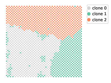
Firstly, <output_dir>/clone3_rectangle0_w1.0/plots/clone_spatial.pdf shows the inferred cancer clone in space.
from wand.image import Image as WImage
img = WImage(filename=f"{output_dir}/clone3_rectangle0_w1.0/plots/clone_spatial.pdf", resolution=100)
img
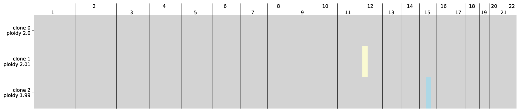
Secondly, <output_dir>/clone3_rectangle0_w1.0/plots/acn_genome.pdf shows the allele-specific copy numbers per clone along the genome. The color scheme follows
# allele-specific copy numbers of each clone (the color scheme is the same as Fig2c
img = WImage(filename=f"{output_dir}/clone3_rectangle0_w1.0/plots/acn_genome.pdf", resolution=120)
img
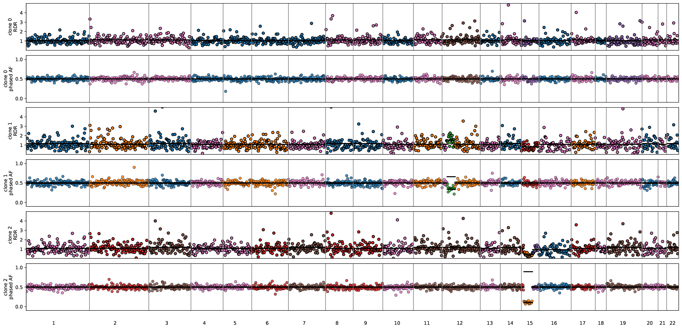
Thirdly, <output_dir>/clone3_rectangle0_w1.0/plots/rdr_baf_defaultcolor.pdf shows RDR-BAF along the genome for each clone. Here, each color indicates a HMM state, while different colors may correspond to the same allele-specific copy numbers.
# RDR-BAF plot along the genome for each clone
img = WImage(filename=f"{output_dir}/clone3_rectangle0_w1.0/plots/rdr_baf_defaultcolor.pdf", resolution=120)
img